
Value at Risk (VaR)
It is defined as the worst loss that could occur over a given period of time under normal circumstances.

Updated:
June 19, 2023Value at Risk (VaR) is the worst loss that could occur over a given period of time under normal circumstances. It can also be described as the maximum loss estimated to be possible, given a certain level of certainty.

Investment and commercial banks frequently use this indicator to assess the size and likelihood of prospective losses in their institutional portfolios.
The confidence level indicates the possibility of acquiring a value greater than or equal to Val. Any predetermined time, expressed in days, weeks, months, or years, can be used as the holding period.
It is a tool used by risk managers to gauge and manage the degree of risk exposure. Its calculations can be used to assess individual holdings, entire portfolios, or the overall risk exposure of an organization.
It is defined as the highest monetary loss that may reasonably be anticipated over a specified time horizon with a particularconfidence level.
A portfolio will not lose more than $1 million over the course of the following month, for instance, if the 95% one-month VaR is $1 million.

Due to the possibility of individual trading desks inadvertently exposing the business to highly-correlated assets, investment banks usually use VaR modeling to assess firm-wide risk.
With elliptical return distributions, like the normal distribution, VaR measurements tend to perform well. The risk for non-normal distributions can also be calculated using this, although the results may not be as accurate.
What is Value at Risk (VaR)?
Volatility is the most widely used and established method of measuring risk. The primary issue with volatility is that it doesn't care which way an investment moves; for example, a stock can be volatile if it suddenly climbs higher.

It is based on the idea that investors are worried about the likelihood of losing money.
A VaR statistic consists of three elements:
- Specific percentage or value of the loss
- Period of time during which the risk is evaluated
- Confidence level
It gives managers and investors a view into the worst-case scenario for investment if they are concerned about the likelihood of a significant loss.
The risk for investors is the likelihood of losing money, and it is based on this obvious truth. The question "What is my worst-case scenario?" or "How much could I lose in a truly terrible month?" is answered by this by presuming investors are worried about the likelihood of a really big loss.
VaR modeling is used to calculate an entity's potential for loss as well as the probability that the stated loss will occur. It is calculated by adding up the potential loss sum, the probability that it will happen, and the time range. The risk will vary depending on the level of confidence selected, and as the confidence level rises, the VaR will also rise. Moreover, as the confidence level rises, it will also rise at an increasing rate.

As the holding time lengthens, the value at risk will rise as well. The mean of the distribution plays a role in determining how quickly VaR rises.
If the return distribution has a mean, μ (pronounced mew), equal to 0, then it rises with the square root of the holding period (i.e., the square root of time).
If the return distribution has μ > 0, then the VaR rises at a lower rate andeventually decreasese. Thus, the mean of the distribution is an important determinant for estimating how it changes with changes in the holding period.
Methods Used for Calculating VaR
The historical technique, variance-covariance method, and Monte Carlo Simulation are the three basic approaches used to calculate VaR.

Each has its own set of calculations, assumptions, and benefits and drawbacks relating to complexity, calculation speed, applicability to particular financial instruments, and other elements.
Historical Method
Calculating it is easy and simple when using the historical simulation method. It begins by determining the risk factors, including interest rates, currency exchange rates, stock prices, volatilities, credit spreads, etc.

Then, in most cases, daily data is gathered on these variables, and scenario analysis is employed to simulate daily changes. A portfolio'se daily gains or losses can therefore be calculated using these scenarios. The historical simulation method would then rank these returns from least (biggest losses) to largest (largest gains).
For example, assume that you have calculated the daily returns of security and produced a histogram of this data. You then compute the monthly VaR for this security at a 95% confidence level.
The smaller tail would display the lowest 5% of returns of the underlying distribution's returns, providing a 95% confidence level.
If you have $2,000,000 invested in a security that has a one-day percentage VaR of -14.3%, then the maximum loss that you should expect is $286,000 (-1.43% x $2,000,000).
Suppose you have computed the returns for 300 days and ranked each day by the amount of loss. You want to calculate the VaR over a one-day time horizon with a 99% confidence level (1% significance). You would take the third worst outcome (3 / 300 = 0.01).
| Scenario Number | Loss (In USD millions) |
|---|---|
| 20 | 15.4 |
| 51 | 16.6 |
| 118 | 13.5 |
| 289 | 12.9 |
| 71 | 9.7 |
| 225 | 7.5 |
| … | … |
The one-day VaR in the above case would be USD 13.5 million.
Advantage: The advantage of this approach is that it may identify a crisis event that was previously overlooked for a specific asset class. The focus is on identifying extreme changes in valuation.
Disadvantage: The historical simulation approach is limited to actual historical data.
Variance-Covariance Method
In comparison to the historical method, the variance-covariance method explicitly assumes a distribution for the underlying observations. This method can be used forlinearly dependent portfoliost on the underlying market variables.

This approach assumes that benefits and losses are dispersed equally instead of thinking that the past will guide the future.
Potential losses can, therefore, be described in terms of deviations from the mean by a standard deviation. It is also referred to as the parametric method, and it works well for risk-measuring scenarios where the distributions can be accurately approximated.
A normal distribution curve can be produced by adding the standard deviation and estimated (or average) returns.
Assuming the returns on these variables are multivariate normal, the portfolio value change will be normally distributed. This makes VaR calculations more intuitive.
Formula to calculate:
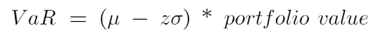
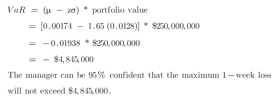
Example: Calculating Value at Risk
For a $250,000,000 portfolio, the expected daily 1-week portfolio return and standard deviation are 0.00174 and 0.0128, respectively. So how do we calculate the 1-week VaR with a 95% confidence level?
Estimated (or average) returns and standard deviation can be combined to create a normal distribution curve.
The variance-covariance approach is conceptually identical to the historical approach, except that we employ the well-known curve rather than actual data.
The benefit of the normal curve is that it tells us where the worst 5% and 1% of the data are located. They depend on the standard deviation and the desired level of confidence.
Advantage: Using a normal distribution curve gives a clear overview of the most likely return on an asset. With the normal distribution curve formed, it is fairly easy to determine the probability of a certain return occurring.
Disadvantage: The normal distribution may not be realistic. Off-market factors can increase price volatility, resulting in the normal distribution curve being out of sync with actual market conditions.
Monte Carlo Method
The Monte Carlo method simulates millions of valuation options for the underlying assets and generates scenarios using random samples.

It entails creating a model to predict future stock price returns and putting it through numerous fictitious trials. Any technique that generates trials at random is referred to as a Monte Carlo simulation, but the term itself does not reveal anything about the underlying process.
A Monte Carlo simulation is essentially a "black box" generator of random, probabilistic results for most users.
The Monte Carlo approach involves six steps:
- Calculate the portfolio's current value using the risk factors' current values.
- For the change in x (Δxi), use sampling procedures from the multivariate normal probability distribution.
- Find the risk factor values at the end of the period using the sampled values.
- Utilize the most recent risk factor values to revalue the portfolio.
- Subtract the portfolio's revalued value from its present value. The degree of the loss will depend on this.
- To generate a loss distribution, repeat steps two through five.
Once this process is complete, we can calculate daily VaR and expected loss using an approach similar to historical simulation.
For example, if a Monte Carlo model produces 1000 trials, the daily VaR with a 99% confidence level will be the tenth worst loss (=1% x 1000), and the expected loss will be the average of the four worst losses.
Remember, to calculate longer-period VaR and expected losses, the daily values will be multiplied by the square root of time.
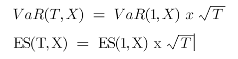
Where:
T= T - (day) time horizon
Advantage: It can address many risk factors by assuming an underlying distribution and simulating the correlations between the risk components.
For instance, a risk manager can simulate 1000 events and then calculate the likelihood that a particular event would occur.
The risk manager only needs to supply parameters for the mean and standard deviation and assume that all potential outcomes are normally distributed in order to perform the simulations.
Using any distribution type with the Monte Carlo simulation is a big advantage, provided the correlation between the risk components can be established.
Disadvantage: The method's main drawback is how slowly and computationally demanding it is. The time-consuming Monte Carlo technique is frequently used for large portfolios.
Limitations of Value at Risk
The main drawback of the VaR measure of risk is the calculation's use of two arbitrary parameters, the holding duration, and the confidence level.

Model risk and implementation risk can affect VaR calculations. Model risk is the possibility of mistakes resulting from inaccurate model assumptions. The danger of mistakes occurring during model implementation is known as implementation risk.
The VaR measure's inability to communicate to the investor the size or scope of the actual loss is another significant flaw. VaR provides only the maximum value we could lose for a particular confidence level.
Two different return distributions may have the same VaR but very different risk exposures. A practical example of how this can be a serious problem is when a portfolio manager sells out-of-the-money options.
For the majority of the time, the options will have a positive return, and, therefore, the expected return is positive. However, in the unfavorable event that the options expire out of the money, the resulting loss can be very large. Thus, different strategies focusing on lowering VaR can be very misleading since the magnitude of the loss is not calculated.
- VaR is a tool used by risk managers to gauge and manage the degree of risk exposure. For example, it is used to assess individual holdings, entire portfolios, or the overall risk exposure of an organization.
- There are several methods to calculate value at risk, including historical, variance-covariance, and Monte Carlo methods.
- VaR modeling is used to calculate the entity's potential for loss and the probability that the stated loss will occur.
- This metric gives managers and investors a view into the worst-case scenario for investment if they are concerned about the likelihood of a significant loss.

Everything You Need To Master Excel Modeling
To Help You Thrive in the Most Prestigious Jobs on Wall Street.

or Want to Sign up with your social account?